How to Use Excel to Project Your Savings – Part 1

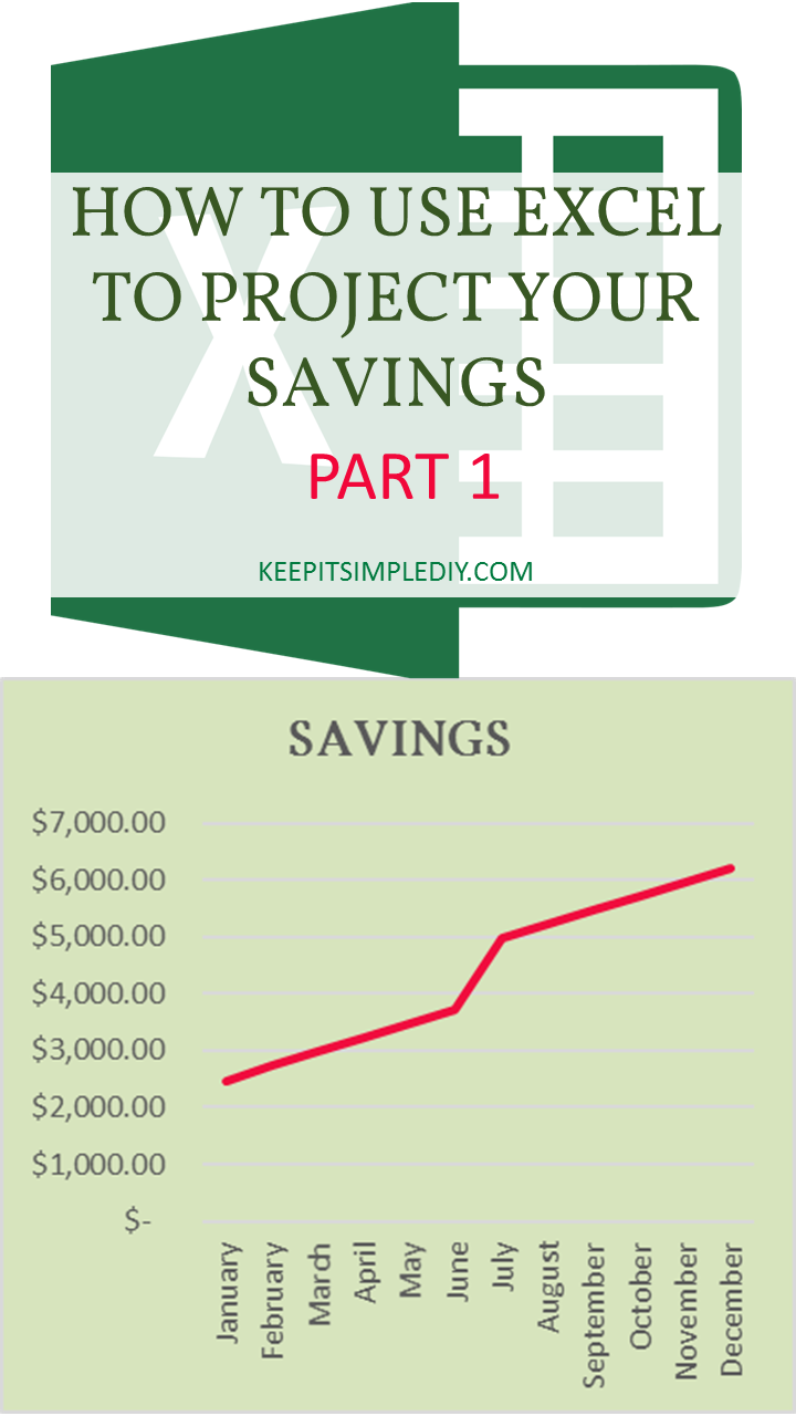
Today I will be showing you “How to Use Excel to Project Your Savings- Part 1”.

For this example, we will begin our projections in January and end in December.  We will assume that income is received twice per month and that expenses include ‘Rent’, ‘Water’, ‘Electricity’, ‘Phone’, ‘Internet’, and ‘Incidentals’ which could be groceries, gas, entertainment, etc.

Let’s start by opening a new document in Microsoft Excel.  We will begin by entering our projection period.

In cell B1, type ‘January’.  By hovering to the bottom right corner of the cell, you will be able to click and drag the cell to the right until you reach M1.  Excel will automatically fill the series through December.

Next, much like an income statement, we will note our ‘Income’ and ‘Expenses’.   In Cell A2, type ‘Income’ then hit ‘Enter’ to go down a line.  Enter both paychecks on separate lines and then total the income below.  Expenses are entered using the same process.

I like to add some formatting at this point so I can navigate easily.  Click the square to the left of the ‘A’ Column and above the ‘1’ Row to highlight all cells then click between the ‘A’ and ‘B’ column to adjust the cells to fit the text.   Next, I bold the headers by highlighting the rows and using CTRL B.  Now we have the basic structure for our projections.

Let’s assume that each paycheck received is $750 and enter this into both cells B3 and B4.  In B5 we will use the sum function to add the two rows paychecks together.  I like to type ‘=sum(‘ and then highlight the cells I want to sum, but there are many options.  Notice that the total income for January is in bold.  Because I have my spreadsheet set to accounting, my numbers came up with dollar signs.  If yours do not, highlight the entire spreadsheet again then click the dollar sign under Home: Number.

Now enter in the expenses and sum the total.  We will assume the following:

Rent: $500; Water $50; Electricity $75; Phone $75; Internet $50; Incidentals $300.

I summed all of my expenses prior to adding in the incidental amount to ensure that I didn’t have a negative balance in my example.  It is not necessary to wait to enter this amount.

Now that we have all of January’s Income and Expenses into our spreadsheet, we will determine how much money is left after all of the expenses have been paid.  For the example, let’s assume all additional funds will be saved.

Type ‘Savings’ in cell A16 then tab to B16.  In A17, we want to subtract our expenses from our income.  There are many ways to do this, but my preference is to type the equals sign, then click on the total income, type the minus sign, click on the total expenses, then hit ‘Enter’.  This shows us that the total savings for the month is $450.

To take this a step further, we will keep a running total of the expenses throughout the year.  I labeled my running total ‘Accumulated Expenses’ then called the cell above by typing = then clicking on cell A16.

Next, we will fill our numbers to the right and let Excel do the work for us.  To do this, highlight cells B3:B17; all cells with an amount.  Like we did with the months, hover towards the bottom right corner of the cell the click and drag all the way to the M column.   If needed, highlight all and expand the cells.

You will notice that our ‘Accumulated Savings’ column remained $450 through the entire spreadsheet.  This is because we only called our savings total and not any totals from previous months.  To update this line, we will begin in February, C17, and add February’s savings amount to the amount saved in January.  ‘=C16+B17’.  Now fill the equation from C17 to M17.

I like to add colors to all of my spreadsheets to keep them easy to read at a glance but this is not necessary.  Now that the projection is complete, a simple glance at the month’s accumulated savings will show how much money is available and allow for planning of large purchases or more saving.  Who doesn’t like watching those numbers grow!?