

Let’s begin by labeling our tabs. I’ve labeled our current worksheet ‘Projections’ and then labeled a new worksheet ‘Checking’.
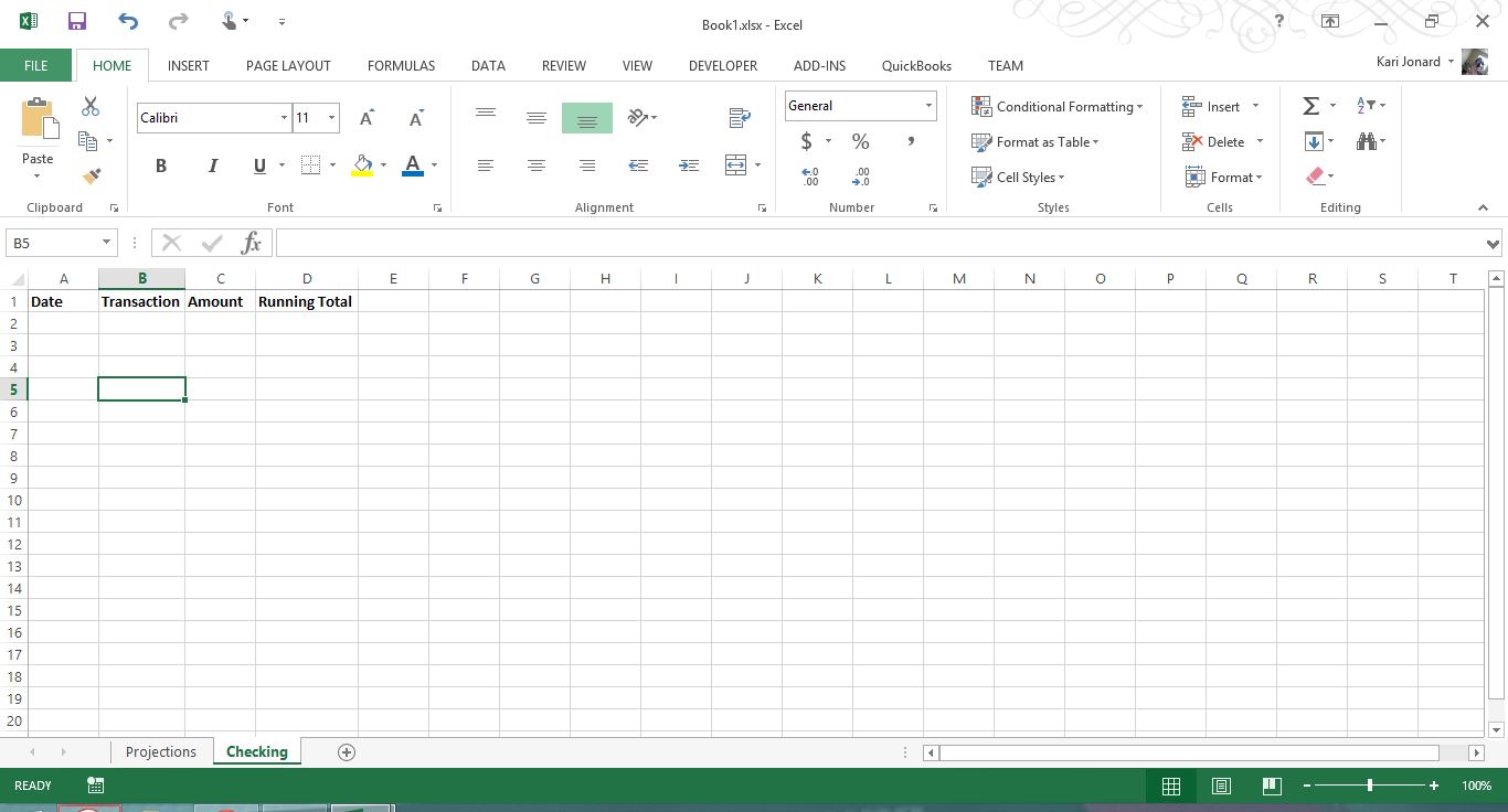
Open the Checking account tab and begin by building the headers. I started my labels in cell A1 and used the following labels:
A1: Date
B1: Transactions
C1: Amount
D1: Running Total
I also made my row 1 Bold because I find it easier to read the table if my headers are bold.
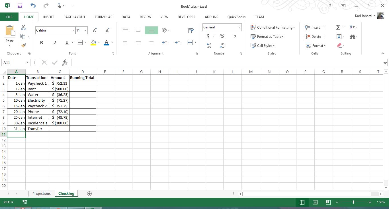
From there, we will add the information from our ‘Projections’ tab into our checking account. It is assumed that all transactions that occur throughout the month are done through the checking account.
The order of the transactions here doesn’t need to match the order of the transactions in the projection’s tab. Use the transaction date to create the order for your transactions.
To enter the amounts, I use a function rather than entering them by hand to avoid errors in typing. For income, I type the equals sign, click on the projections tab, then click the cell I want.
- For Paycheck 1, the equation would look like this: =Projections!B3
For expenses, I use the same process but add a negative before clicking projections so the amounts will be debited from the account
- For January’s Rent, the equation would look like this: =-Projections!B8
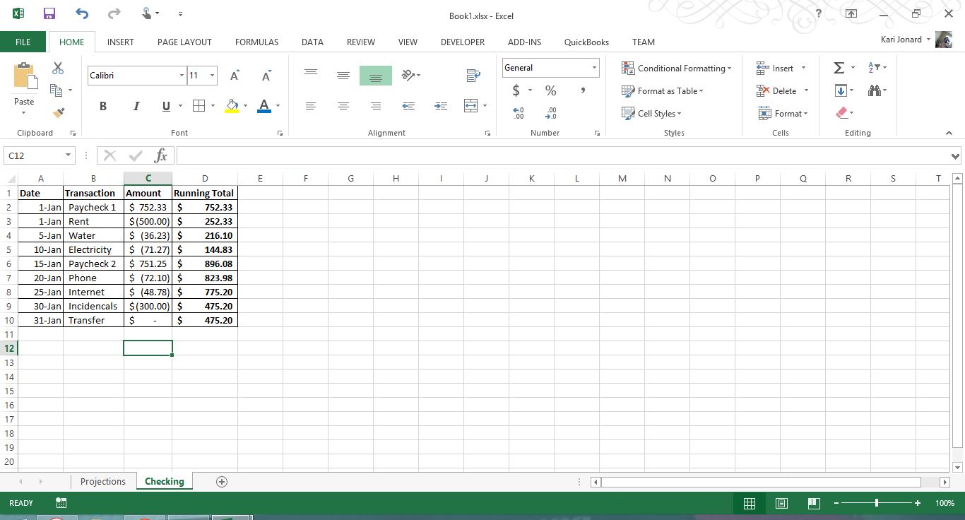
To fill in the running total (I made all of column D bold), we need to start by pulling our first transaction. To do this, type the equals sign, then click on C2 in the same tab. You can also type the equation =C2. This is the only cell you will use this equation.
In cell D3, type =D2+C3 or click on the cells to add the cell numbers to the equation. This will take the previous balance in the checking account and the new transaction. Fill down using the methods discussed earlier in the excel budgeting series to complete your running totals.
Make sure that your end balance for the month is the same as the end balance for the month in the Projections tab. (This example’s end balance is $475.20). If they are not the same, your account does not balance and the transactions need to be double checked for accuracy.
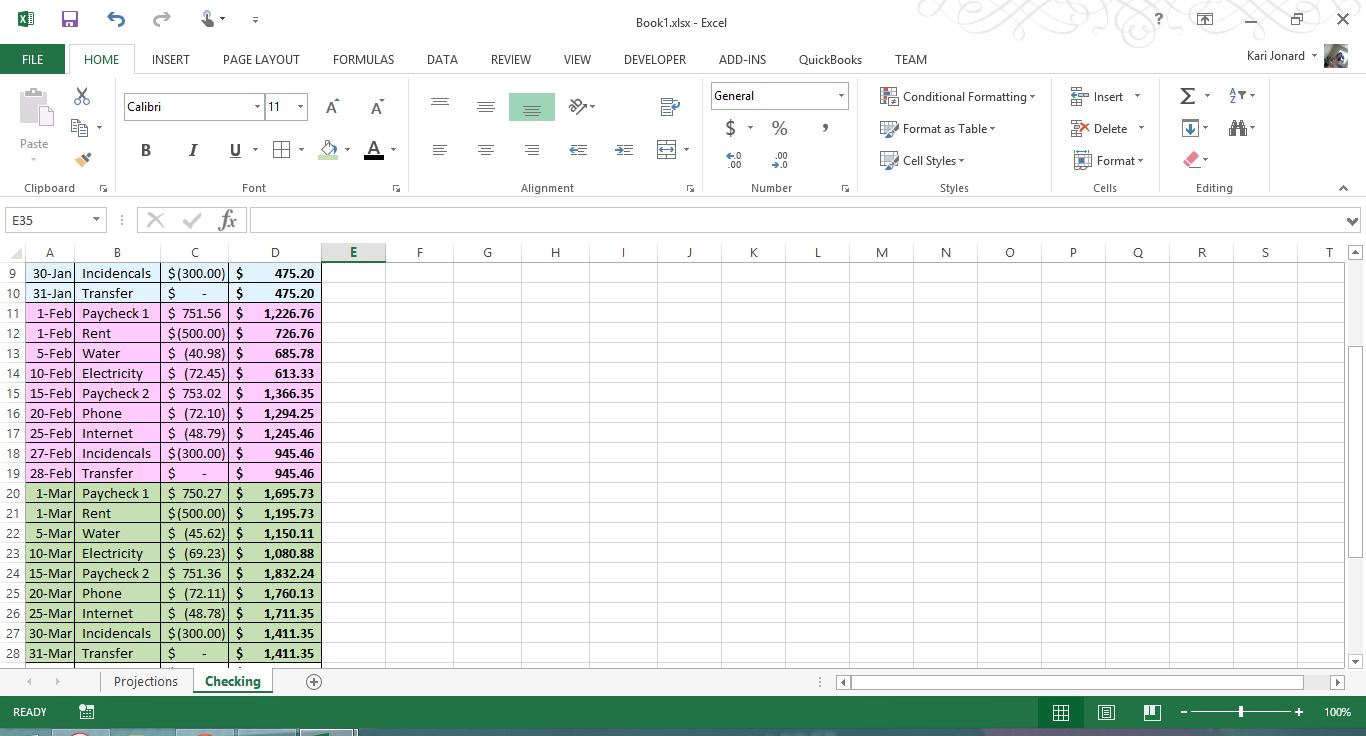
Use the same process to add additional months, making sure to double check your totals. In the above example, I added February and March. Next week, I will show how to include the transfer to the savings account that happens in April of our example.
Side Note: I also like to use colors to separate my months so I can quickly glance and see the entire month.